Wind Spectral Analysis for the FAST Radio Telescope
A Python prototype that turns time-stamped wind records from several anemometers at the FAST radio telescope into along-wind and cross-wind power spectra. Its plots were the reference for a later Java implementation in the telescope's operations system.
- Period
- Jan–Mar 2026
- Context
- Internship, Architectural Design and Research Institute, Chinese Academy of Sciences
- Team
- Individual project
- My role
- Algorithm engineer intern; author of the Python prototype
- Status
- Prototype delivered during the internship and used as the reference for the Java implementation
Demo & artifacts
- Open demoSimulated data
The walkthrough runs in your browser on simulated wind records. You choose the input and processing options, then watch each step with the matching lines of the original script highlighted. An optional button runs the unmodified Python file with Pyodide (about 25 MB download) and compares the results. It does not connect to telescope data.
My contribution
- Wrote a per-device Python pipeline with pandas, NumPy and SciPy. It reads time-stamped speed and 16-sector direction records, groups them by device and sorts each device by time.
- Estimated each device's sampling rate from the median timestamp interval, so devices with different rates need no hard-coded value and a few irregular intervals do not shift the estimate.
- Converted the 16 direction sectors to angles, turned the wind-from convention into the direction the air moves, and resolved every sample into along-wind and cross-wind components relative to the mean wind direction.
- Removed the means and estimated one-sided power spectral densities with Welch's method, using a 1,024-sample periodic Hann window with 50 % overlap; the code notes the MATLAB equivalent of each setting. The script saves six plots per device (three spectra, each on log-log and linear-frequency axes) as the reference for the Java/JTransforms implementation.
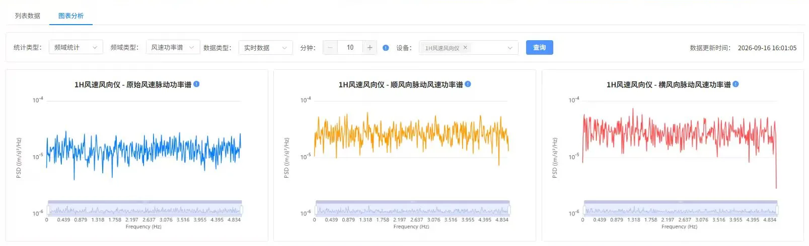
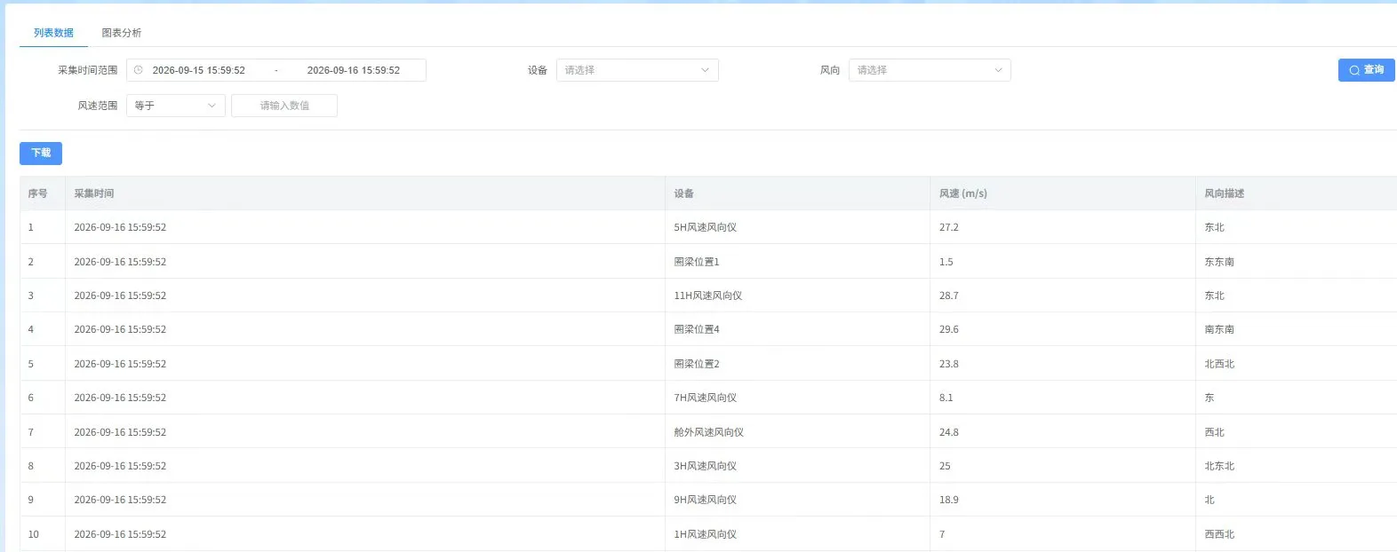
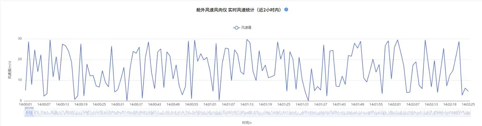
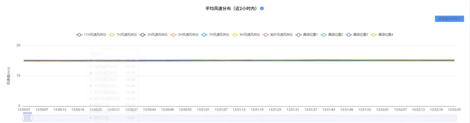
The prototype was my own work within the institute's project. The Java service, database jobs and web pages in the screenshots belong to the wider operations system. They are shown to explain where the spectra are used, not as my work.
Why wind spectra at FAST
FAST, the Five-hundred-meter Aperture Spherical radio Telescope in Guizhou, China, suspends its receiver cabin from six cables high above the dish, and several anemometers around the site record wind speed and direction. A mean speed does not say how gusty the wind is. A power spectrum does: it shows how the energy of the speed fluctuations is spread across frequencies. Splitting the wind into a component along the mean direction and one across it shows the two separately.
How it works
The script runs the same chain for every device in the file. The sampling rate is estimated per device, so a 4 Hz and a 10 Hz anemometer can share one input. Directions are averaged as vectors, not angles, because 350° and 10° should average to north, not south. Welch’s method then cuts each fluctuation series into overlapping 1,024-sample windows, applies a Hann window to each, and averages their periodograms. A single FFT of the whole record would be much noisier.
The walkthrough runs each of these steps with the matching lines of the script highlighted, and shows the intermediate values.
What re-checking the script showed
When I ported the script for the walkthrough, I checked each step against cases with a known answer. Two problems came up that the plots alone would never reveal.
A 90° slip that cancels out. Wind direction is a compass bearing, clockwise from north. The script negates it and adds 180°, but then uses the result as a mathematical angle, which is measured from east. Wind from the north therefore comes out as blowing towards the west instead of the south:
theta = -dir_deg                      # still measured from north
theta = np.deg2rad(theta) + np.pi
u_east = speed * np.cos(theta)        # ...but used as if measured from east

# corrected: bearing -> angle from east, then wind-from -> wind-to
theta = np.deg2rad(90.0 - dir_deg) + np.pi
The spectra are still right. Every vector is rotated by the same 90°, so the mean direction rotates with them, and projecting onto along-wind and cross-wind axes gives the same numbers. In my test, the along-wind and cross-wind spectra from the two conversions agreed to within rounding error (about 10⁻¹⁵ relative). The east and north components and the implied mean direction are wrong, though, and they would matter as soon as anything reports a direction. The walkthrough shows the slip in step 3 and the cancellation in step 5.
Gaps that shift peaks. Taking the median timestamp interval keeps a few long gaps from distorting the rate, which was the reason for choosing it. Missing samples are still treated as if they were consecutive, though. In the walkthrough, with 8 % of samples missing, a 0.5 Hz sine shows up at 0.54 Hz using the median rate. The Java notes’ (N − 1)/time span moves it back to 0.50 Hz but leaves it as low and broad as before. Interpolating onto a uniform grid first gives a peak about six times higher, at 0.50 Hz. Neither rate formula fixes the gaps on its own; the data has to be made evenly spaced first.
Results & validation
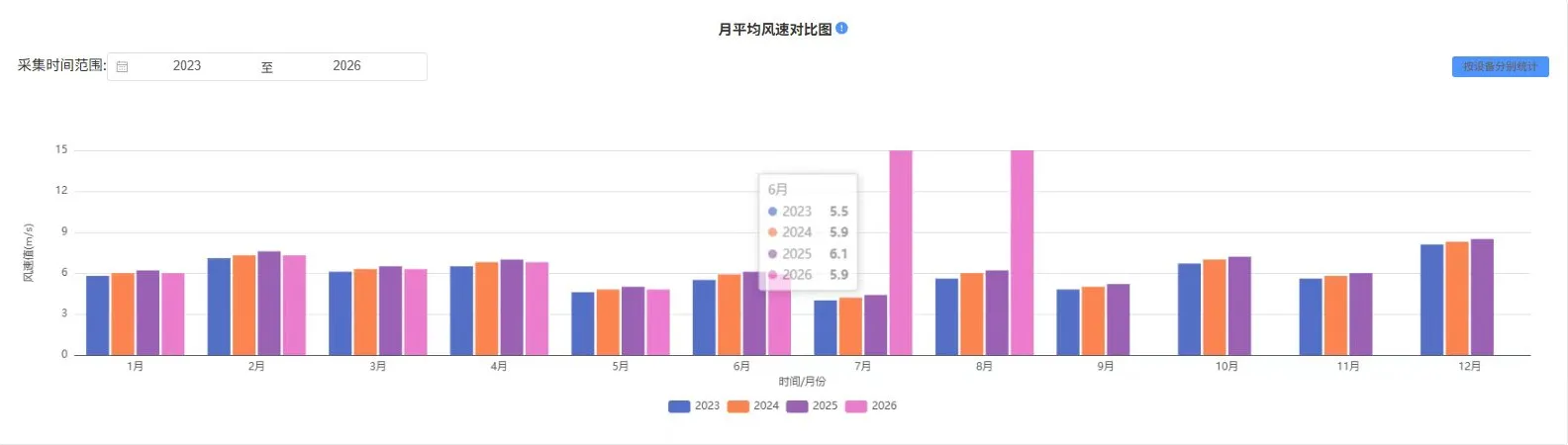
- Delivered the prototype and its per-device plots during the internship. The operations system's frequency-domain view (cover screenshot) shows the same three spectra.
- For this page I ported the script to TypeScript. On three simulated records (10 Hz and 4 Hz, with and without gaps), its spectra agree with the original script running on SciPy 1.18 to within 1.7 × 10⁻¹⁴ relative difference on every frequency bin. A fourth, too-short record stops with the same SciPy error in both. (Pyodide's older SciPy 1.14 words that error differently, and the walkthrough accepts either wording.)
- The walkthrough can run the unmodified
cal_wind.pyin the browser with Pyodide and repeats this bin-by-bin comparison on whatever input you choose. - Re-checking the script turned up two issues that the plots do not show: a 90° slip in the direction conversion, and uneven sampling when records have gaps. Both are explained below and listed under next steps.
The archived script reads a simulated data file (simulated_winddata.csv), and no telescope wind data is published here. The screenshots come from a test environment and their values appear to be test data. The comparison with SciPy was run for this website in November 2026.
Limitations & next steps
- Direction conversion: the script computes θ = −bearing + 180° but then treats θ as measured from east. Its east and north components, and any mean direction taken from them, are therefore rotated 90° clockwise. The three spectra are unaffected. Fix: θ = 90° − bearing + 180°, plus a unit test with known directions (wind from the north must blow towards the south).
- Gaps: Welch's method assumes evenly spaced samples. The median interval gives the nominal rate, but missing samples are still treated as consecutive. With 8 % of samples missing, a 0.5 Hz sine appears at 0.54 Hz. Next step: interpolate onto a uniform grid, or reject windows with gaps, before the FFT. The walkthrough compares both rate estimates with resampling.
- Matching the Java version: the Java design notes use (N − 1)/time span for the rate and remove each segment's mean, and their calculator class fixes
nfftat 1,024 (their parameter table gives the script's rule). The script does none of these. The notes also give a symmetric Hann formula for a window described as periodic. These settings must match before the two implementations can be compared. - Minimum length: with
nperseg= 1,024 and the script'snfftrule, records of 1,024 samples or fewer (about 100 s at 10 Hz, 256 s at 4 Hz) stop with a SciPy error instead of a clear message. - Direction resolution: directions are stored as 16 sectors of 22.5°, so small direction changes are lost and jumps between sectors add power across the cross-wind spectrum. The walkthrough lets you compare 16 sectors with exact angles.
- No uncertainty is reported. A 10-minute record at 10 Hz gives only 10 Welch segments, so each spectral value has wide confidence limits.
Run / reproduce
Environment
- Python 3 with NumPy, pandas, SciPy and Matplotlib
- A CSV named
simulated_winddata.csvwith columnsts(seconds),dev_code,wind_speed(m/s) andwind_dir(sector 0–15)
Steps
- In the walkthrough, choose an input and use “Download input CSV” and “Download cal_wind.py”.
- Put both files in one folder and run
python cal_wind.py. - Six PNG files per device appear in
psd_figures/. “Download spectra CSV” gives the same values for comparison.
The script has no repository; its full text is shown and downloadable in the walkthrough.